35. Optimal Growth II: Time Iteration#

35.2.1. The Coleman Operator#

Recall the Bellman operator

Just as we introduced the Bellman operator to solve the Bellman equation, we will now introduce an operator over policies to help us solve the Euler equation.

This operator $K$ will act on the set of all $\sigma \in \mathrm{\Sigma }$ that are continuous, strictly increasing and interior (i.e., $0<\sigma (y)<y$ for all strictly positive $y$).

Henceforth we denote this set of policies by $\mathcal{P}$

1. The operator $K$ takes as its argument a $\sigma \in \mathcal{P}$ and

2. returns a new function $K\sigma$, where $K\sigma (y)$ is the $c\in (0,y)$ that solves

We call this operator the Coleman operator to acknowledge the work of [Col90] (although many people have studied this and other closely related iterative techniques).

In essence, $K\sigma$ is the consumption policy that the Euler equation tells you to choose today when your future consumption policy is $\sigma$.

The important thing to note about $K$ is that, by construction, its fixed points coincide with solutions to the functional equation (35.5).

In particular, the optimal policy $c^{\ast }$ is a fixed point.

Indeed, for fixed $y$, the value $K{c}^{\ast }(y)$ is the $c$ that solves

In view of the Euler equation, this is exactly $c^{\ast }(y)$.

35.2.2. Is the Coleman Operator Well Defined?#

In particular, is there always a unique $c\in (0,y)$ that solves (35.7)?

The answer is yes, under our assumptions.

For any $\sigma \in \mathcal{P}$, the right side of (35.7)

• is continuous and strictly increasing in $c$ on $(0,y)$

• diverges to $+\mathrm{\infty }$ as $c\uparrow y$

The left side of (35.7)

• is continuous and strictly decreasing in $c$ on $(0,y)$

• diverges to $+\mathrm{\infty }$ as $c\downarrow 0$

Sketching these curves and using the information above will convince you that they cross exactly once as $c$ ranges over $(0,y)$.

With a bit more analysis, one can show in addition that $K\sigma \in \mathcal{P}$ whenever $\sigma \in \mathcal{P}$.

35.3.1. Equivalent Dynamics#

Let’s talk about the theory first.

To explain the connection between the two algorithms, it helps to understand the notion of equivalent dynamics.

(This concept is very helpful in many other contexts as well).

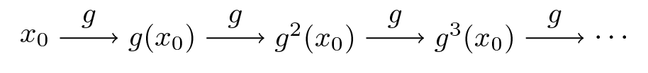
Suppose that we have a function $g:X\to X$ where $X$ is a given set.

The pair $(X,g)$ is sometimes called a dynamical system and we associate it with trajectories of the form

Equivalently, $x_t=g^t(x_0)$, where $g$ is the $t$-th composition of $g$ with itself.

Here’s the picture

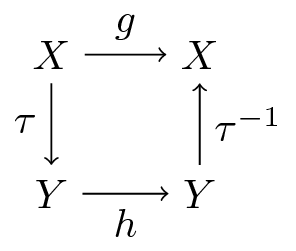
Now let another function $h:Y\to Y$ where $Y$ is another set.

Suppose further that

• there exists a bijection $\tau$ from $X$ to $Y$

• the two functions commute under $\tau$, which is to say that $\tau (g(x))=h(\tau (x))$ for all $x\in X$

The last statement can be written more simply as

or, by applying ${\tau }^{-1}$ to both sides

Here’s a commutative diagram that illustrates

Here’s a similar figure that traces out the action of the maps on a point $x\in X$

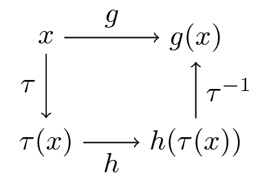
Now, it’s easy to check from (35.8) that $g^2={\tau }^{-1}\circ h^2\circ \tau$ holds.

In fact, if you like proofs by induction, you won’t have trouble showing that

is valid for all $n$.

What does this tell us?

It tells us that the following are equivalent

• iterate $n$ times with $g$, starting at $x$

• shift $x$ to $Y$ using $\tau$, iterate $n$ times with $h$ starting at $\tau (x)$, and shift the result $h^n(\tau (x))$ back to $X$ using ${\tau }^{-1}$

We end up with exactly the same object.

35.3.2. Back to Economics#

Have you guessed where this is leading?

What we’re going to show now is that the operators $T$ and $K$ commute under a certain bijection.

The implication is that they have exactly the same rate of convergence.

To make life a little easier, we’ll assume in the following analysis (although not always in our applications) that $u(0)=0$.

35.4.1. The Operator#

Here’s some code that implements the Coleman operator.

using LinearAlgebra, Statistics
using BenchmarkTools, Interpolations, LaTeXStrings,  Plots, Roots
using Optim, Random

using BenchmarkTools, Interpolations, Plots, Roots

function K!(Kg, g, grid, beta, dudc, f, f_prime, shocks)
    # This function requires the container of the output value as argument Kg

    # Construct linear interpolation object
    g_func = LinearInterpolation(grid, g, extrapolation_bc = Line())

    # solve for updated consumption value
    for (i, y) in enumerate(grid)
        function h(c)
            vals = dudc.(g_func.(f(y - c) * shocks)) .* f_prime(y - c) .* shocks
            return dudc(c) - beta * mean(vals)
        end
        Kg[i] = find_zero(h, (1e-10, y - 1e-10))
    end
    return Kg
end

# The following function does NOT require the container of the output value as argument
function K(g, grid, beta, dudc, f, f_prime, shocks)
    K!(similar(g), g, grid, beta, dudc, f, f_prime, shocks)
end

K (generic function with 1 method)

It has some similarities to the code for the Bellman operator in our optimal growth lecture.

For example, it evaluates integrals by Monte Carlo and approximates functions using linear interpolation.

Here’s that Bellman operator code again, which needs to be executed because we’ll use it in some tests below

using Optim

function T(w, grid, beta, u, f, shocks, Tw = similar(w);
           compute_policy = false)

    # apply linear interpolation to w
    w_func = LinearInterpolation(grid, w, extrapolation_bc = Line())

    if compute_policy
        sigma = similar(w)
    end

    # set Tw[i] = max_c { u(c) + beta E w(f(y  - c) z)}
    for (i, y) in enumerate(grid)
        objective(c) = u(c) + beta * mean(w_func.(f(y - c) .* shocks))
        res = maximize(objective, 1e-10, y)

        if compute_policy
            sigma[i] = Optim.maximizer(res)
        end
        Tw[i] = Optim.maximum(res)
    end

    if compute_policy
        return Tw, sigma
    else
        return Tw
    end
end

T (generic function with 2 methods)

35.4.2. Testing on the Log / Cobb–Douglas case#

As we did for value function iteration, let’s start by testing our method in the presence of a model that does have an analytical solution.

Here’s an object containing data from the log-linear growth model we used in the value function iteration lecture

isoelastic(c, gamma) = isone(gamma) ? log(c) : (c^(1 - gamma) - 1) / (1 - gamma)
function Model(; alpha = 0.65,                         # Productivity parameter
               beta = 0.95,                            # Discount factor
               gamma = 1.0,                             # Risk aversion
               mu = 0.0,                             # First parameter in lognorm(mu, sigma)
               s = 0.1,                             # Second parameter in lognorm(mu, sigma)
               grid = range(1e-6, 4, length = 200), # Grid
               grid_min = 1e-6,                     # Smallest grid point
               grid_max = 4.0,                      # Largest grid point
               grid_size = 200,                     # Number of grid points
               u = (c, gamma = gamma) -> isoelastic(c, gamma),  # utility function
               dudc = c -> c^(-gamma),                  # u_prime
               f = k -> k^alpha,                        # production function
               f_prime = k -> alpha * k^(alpha - 1))
    return (; alpha, beta, gamma, mu, s, grid, grid_min, grid_max, grid_size, u,
            dudc, f, f_prime)
end

Model (generic function with 1 method)

Next we generate an instance

m = Model();

We also need some shock draws for Monte Carlo integration

using Random
Random.seed!(42) # for reproducible results.

shock_size = 250 # number of shock draws in Monte Carlo integral
shocks = collect(exp.(m.mu .+ m.s * randn(shock_size))); # generate shocks

As a preliminary test, let’s see if $K{c}^{\ast }=c^{\ast }$, as implied by the theory

function verify_true_policy(m, shocks, c_star)
    # compute (Kc_star)
    (; grid, beta, dudc, f, f_prime) = m
    c_star_new = K(c_star, grid, beta, dudc, f, f_prime, shocks)

    # plot c_star and Kc_star
    plot(grid, c_star, label = L"optimal policy $c^*$")
    plot!(grid, c_star_new, label = L"Kc^*")
    plot!(legend = :topleft)
end

verify_true_policy (generic function with 1 method)

c_star = (1 - m.alpha * m.beta) * m.grid # true policy (c_star)
verify_true_policy(m, shocks, c_star)

We can’t really distinguish the two plots, so we are looking good, at least for this test.

Next let’s try iterating from an arbitrary initial condition and see if we converge towards $c^{\ast }$.

The initial condition we’ll use is the one that eats the whole pie: $c(y)=y$

function check_convergence(m, shocks, c_star, g_init; n_iter = 15)
    (; grid, beta, dudc, f, f_prime) = m
    g = g_init
    plot(m.grid, g, lw = 2, alpha = 0.6, label = L"intial condition $c(y) = y$")
    for i in 1:n_iter
        new_g = K(g, grid, beta, dudc, f, f_prime, shocks)
        g = new_g
        plot!(grid, g, lw = 2, alpha = 0.6, label = "")
    end
    plot!(grid, c_star, color = :black, lw = 2, alpha = 0.8,
          label = L"true policy function $c^*$")
    plot!(legend = :topleft)
end

check_convergence (generic function with 1 method)

check_convergence(m, shocks, c_star, m.grid, n_iter = 15)

We see that the policy has converged nicely, in only a few steps.

Now let’s compare the accuracy of iteration using the Coleman and Bellman operators.

We’ll generate

1. $K^{n}c$ where $c(y)=y$

2. $(M\circ T^n\circ M^{-1})c$ where $c(y)=y$

In each case we’ll compare the resulting policy to $c^{\ast }$.

The theory on equivalent dynamics says we will get the same policy function and hence the same errors.

But in fact we expect the first method to be more accurate for reasons discussed above

function iterate_updating(func, arg_init; sim_length = 20)
    arg = arg_init
    for i in 1:sim_length
        new_arg = func(arg)
        arg = new_arg
    end
    return arg
end

function compare_error(m, shocks, g_init, w_init; sim_length = 20)
    (; grid, beta, u, dudc, f, f_prime) = m
    g, w = g_init, w_init

    # two functions for simplification
    bellman_single_arg(w) = T(w, grid, beta, u, f, shocks)
    coleman_single_arg(g) = K(g, grid, beta, dudc, f, f_prime, shocks)

    g = iterate_updating(coleman_single_arg, grid, sim_length = 20)
    w = iterate_updating(bellman_single_arg, u.(grid), sim_length = 20)
    new_w, vf_g = T(w, grid, beta, u, f, shocks, compute_policy = true)

    pf_error = c_star - g
    vf_error = c_star - vf_g

    plot(grid, zero(grid), color = :black, lw = 1, label = "")
    plot!(grid, pf_error, lw = 2, alpha = 0.6, label = "policy iteration error")
    plot!(grid, vf_error, lw = 2, alpha = 0.6, label = "value iteration error")
    plot!(legend = :bottomleft)
end

compare_error (generic function with 1 method)

compare_error(m, shocks, m.grid, m.u.(m.grid), sim_length = 20)

As you can see, time iteration is much more accurate for a given number of iterations.

35.5.1. Exercise 1#

Show that (35.9) is valid. In particular,

• Let $v$ be strictly concave and continuously differentiable on $(0,\mathrm{\infty })$

• Fix $y\in (0,\mathrm{\infty })$ and show that $MTv(y)=KMv(y)$

35.5.2. Exercise 2#

Show that $M$ is a bijection from $\mathcal{V}$ to $\mathcal{P}$.

35.5.3. Exercise 3#

Consider the same model as above but with the CRRA utility function

Iterate 20 times with Bellman iteration and Euler equation time iteration

• start time iteration from $c(y)=y$

• start value function iteration from $v(y)=u(y)$

• set $\gamma =1.5$

Compare the resulting policies and check that they are close.

35.5.4. Exercise 4#

Do the same exercise, but now, rather than plotting results, benchmark both approaches with 20 iterations.

35.6.1. Solution to Exercise 1#

Let $T,K,M,v$ and $y$ be as stated in the exercise.

Using the envelope theorem, one can show that $(Tv{)}^{\prime }(y)=u^{\prime }(c(y))$ where $c(y)$ solves

Hence $MTv(y)=(u^{\prime }{)}^{-1}(u^{\prime }(c(y)))=c(y)$.

On the other hand, $KMv(y)$ is the $c(y)$ that solves

We see that $c(y)$ is the same in each case.

35.6.2. Solution to Exercise 2#

We need to show that $M$ is a bijection from $\mathcal{V}$ to $\mathcal{P}$.

To see this, first observe that, in view of our assumptions above, $u^{\prime }$ is a strictly decreasing continuous bijection from $(0,\mathrm{\infty })$ to itself.

It follows that $h$ has the same properties.

Moreover, for fixed $v\in \mathcal{V}$, the derivative $v^{\prime }$ is a continuous, strictly decreasing function.

Hence, for fixed $v\in \mathcal{V}$, the map $Mv=h\circ v^{\prime }$ is strictly increasing and continuous, taking values in $(0,\mathrm{\infty })$.

Moreover, interiority holds because $v^{\prime }$ strictly dominates $u^{\prime }$, implying that

In particular, $\sigma (y):=(Mv)(y)$ is an element of $\mathcal{P}$.

To see that each $\sigma \in \mathcal{P}$ has a preimage $v\in \mathcal{V}$ with $Mv=\sigma$, fix any $\sigma \in \mathcal{P}$.

Let $v(y):={\int }_0^y{u}^{\prime }(\sigma (x))dx$ with $v(0)=0$.

With a small amount of effort you will be able to show that $v\in \mathcal{V}$ and $Mv=\sigma$.

It’s also true that $M$ is one-to-one on $\mathcal{V}$.

To see this, suppose that $v$ and $w$ are elements of $\mathcal{V}$ satisfying $Mv=Mw$.

Then $v(0)=w(0)=0$ and $v^{\prime }=w^{\prime }$ on $(0,\mathrm{\infty })$.

The fundamental theorem of calculus then implies that $v=w$ on ${\mathbb{R}}_{+}$.

35.6.3. Solution to Exercise 3#

Here’s the code, which will execute if you’ve run all the code above

# Model instance with risk aversion = 1.5
# others are the same as the previous instance
m_ex = Model(gamma = 1.5);

function exercise2(m, shocks, g_init = m.grid, w_init = m.u.(m.grid);
                   sim_length = 20)
    (; grid, beta, u, dudc, f, f_prime) = m
    # initial policy and value
    g, w = g_init, w_init
    # iteration
    bellman_single_arg(w) = T(w, grid, beta, u, f, shocks)
    coleman_single_arg(g) = K(g, grid, beta, dudc, f, f_prime, shocks)

    g = iterate_updating(coleman_single_arg, grid, sim_length = 20)
    w = iterate_updating(bellman_single_arg, u.(m.grid), sim_length = 20)
    new_w, vf_g = T(w, grid, beta, u, f, shocks, compute_policy = true)

    plot(grid, g, lw = 2, alpha = 0.6, label = "policy iteration")
    plot!(grid, vf_g, lw = 2, alpha = 0.6, label = "value iteration")
    return plot!(legend = :topleft)
end

exercise2 (generic function with 3 methods)

exercise2(m_ex, shocks, m.grid, m.u.(m.grid), sim_length = 20)

The policies are indeed close.

35.6.4. Solution to Exercise 4#

Here’s the code.

It assumes that you’ve just run the code from the previous exercise

function bellman(m, shocks)
    (; grid, beta, u, dudc, f, f_prime) = m
    bellman_single_arg(w) = T(w, grid, beta, u, f, shocks)
    iterate_updating(bellman_single_arg, u.(grid), sim_length = 20)
end
function coleman(m, shocks)
    (; grid, beta, dudc, f, f_prime) = m
    coleman_single_arg(g) = K(g, grid, beta, dudc, f, f_prime, shocks)
    iterate_updating(coleman_single_arg, grid, sim_length = 20)
end

coleman (generic function with 1 method)

@benchmark bellman(m_ex, shocks)

BenchmarkTools.Trial: 47 samples with 1 evaluation per sample.
 Range (min … max):  105.362 ms … 143.433 ms  ┊ GC (min … max): 3.15% … 13.78%
 Time  (median):     105.795 ms               ┊ GC (median):    3.43%
 Time  (mean ± σ):   107.798 ms ±   7.884 ms  ┊ GC (mean ± σ):  3.89% ±  1.65%

  █                                                              
  █▇▁▅▁▁▁▁▁▁▁▁▁▁▁▁▁▁▁▁▁▁▁▁▁▁▁▁▁▁▁▁▁▁▁▁▁▅▁▁▁▁▁▁▁▁▁▁▁▁▁▁▁▅▁▁▁▁▁▁▅ ▁
  105 ms        Histogram: log(frequency) by time        143 ms <

 Memory estimate: 142.09 MiB, allocs estimate: 151962.

@benchmark bellman(m_ex, shocks)

BenchmarkTools.Trial: 47 samples with 1 evaluation per sample.
 Range (min … max):  105.756 ms … 142.888 ms  ┊ GC (min … max): 3.38% … 13.26%
 Time  (median):     106.057 ms               ┊ GC (median):    3.59%
 Time  (mean ± σ):   108.128 ms ±   7.947 ms  ┊ GC (mean ± σ):  4.05% ±  1.63%

  █                                                              
  █▆▅▅▁▁▁▁▁▁▁▁▁▁▁▁▁▁▁▁▁▁▁▁▁▁▁▁▁▁▁▁▁▁▁▁▁▁▁▅▁▁▁▁▁▁▁▁▁▁▁▁▁▁▁▁▅▁▁▁▅ ▁
  106 ms        Histogram: log(frequency) by time        143 ms <

 Memory estimate: 142.09 MiB, allocs estimate: 151962.